Leveraging Physics-Informed Machine Learning to Empower Genetic Algorithms for Mechanical Systems
André Bianchessi
Advisor: Marcilio Alves
Universidade de São Paulo
Programa de Pós-Graduação em Engenharia Mecânica
2023/12/23
Acknowledgments
I would like to express my sincere gratitude to my advisor, Professor Marcilio Alves, for his invaluable guidance, support, and encouragement throughout this work. His expertise and insights were instrumental in shaping this thesis and propelling me forward.
I am also particularly grateful for my informal co-advisor, Professor Larissa Driemeier, for her guidance in all-things-ML related. I can’t overstate how much her expertise and willingness to share her knowledge were crucial for the success of this work.
Furthermore, I would like to extend my heartfelt thanks to Lucas Barroso Knupp, Felipe Yamaguti, and Thiago Estrela Montenegro for the stimulating discussions and valuable insights they provided throughout my research.
This work really took a village, and I am truly grateful for all the support.
How to read this document
Source Code
All of this work’s source code (including all images, text and code) is available at the github.com/andrebianchessi/msc repository under an MIT open source license.
In this text, references to files at the repository are written as:
/software/filename. For example: /software/mass.h
references the mass.h file, which is under the
software folder at the repository. References to specific
functions/methods/classes are written as function_name
(/software/filename). For example: Mass
(/software/mass.h) references the Mass class definition,
which is under the software folder at the repository.
References to the source code are all hyperlinks when this document is being read digitally (not on printed paper). Thus, accessing this document online is highly recommended.
Read online
The thesis text is written in pandoc, and is compiled into pdf format and also a website. The website can be accessed online at andre.how, and the pdf can be downloaded at andre.how/thesis.pdf.
Acronyms
CMs Crashworthiness models. See sec. 3.1.
COP Crashworthiness Optimization Problem. See sec. 3.2.
DEM Discrete Element Method, i.e. a method to find the time-response of a system comprized of ideal masses, linear springs and linear dampers in which the equations of motion have been determined with Newton’s second law. See sec. 3.3.
E-GA Genetic Algorithm which calculates the quality of each candidate solution by explicitly integrating the ODE in time.
ETI Explicit Time Integration, i.e. numerical method for obtaining approximate solution to time-dependent ordinary differential equation. See sec. 3.4.
FEM Finite Element Method.
GA Genetic Algorithm.
ML Machine Learning.
ODE Ordinary Differential Equation.
P-GA Genetic Algorithm which uses a PIM to calculate the quality of each candidate solution.
PIM Physics Informed Machine Learning Model.
4 Motivation
Optimization algorithms are widely spread in all areas of modern engineering industry. They allow for reduction of costs and increase of the efficiency and effectiveness of solutions. The exponential growth in computational power in recent years has made it feasible for engineers to optimize problems they could not optimize before. Still, the complexity of the problems we tackle increases even faster than the available computational power. Thus, advancements in optimization techniques are also required. In this work, we turn our attention to optimization by Genetic Algorithms (GAs) applied to mechanical systems. These algorithms are based on principles of genetics and evolution, and are well suited for the optimization of problems dealing with a large amount of variables, having multiple local minima.
The caveat GA has is that it needs to constantly evaluate the fitness (i.e. ta score of how good each possible solution is) of each candidate solution in the population (i.e. the set of possible solutions) at every iteration. For example: when using GA to minimize the maximum displacement a structure suffers at a specific load condition, it is necessary to calculate the structure’s displacement multiple times for each iteration of the algorithm. Thus, for expensive fitness functions, the algorithm’s computational cost is proportional to the fitness function’s cost. This might make the algorithm too expensive if the fitness is computed, for example, using an expensive Finite Element Model (FEM) simulation.
With this in mind, many recent studies have looked into using Machine Learning (ML) models in conjunction with GA to increase the efficiency of optimizations of high-cost fitness function problems. The basic idea is to train a model which approximates the fitness function but has a much smaller computational cost; and use it to calculate the fitness in the GA, instead of the original fitness function. We call them metamodels because they are used as approximations to another model, such as a FEM simulation [1]–[5].
The challenge of metamodel-based-GAs is that although metamodels can be used for cheaper evaluation of the fitness function, it can be very expensive to train them; especially when they’re trained with synthetic data generated through numerical simulations, which can be very costly depending on the problem. So, the faster evaluation of the fitness function that they provide might not compensate the added cost that they bring.
Physics-Based Machine Learning is a promising field of research that has been quickly growing, and has already shown great results when used in conjunction with GAs [6], [7]. Physics-Informed Machine Learning Models (PIMs) are Machine Learning models which are trained with physics knowledge embedded into the loss function. This allows them to be trained without labeled data. Thus, it’s possible to train, for example, a metamodel to a physical problem without needing to run a numerical simulation multiple times beforehand to obtain training data. This way, PIMs might be good candidates to GAs applied to problems which have expensive fitness functions. Also, given that they’re trained without labeled data, PIMs might have good extrapolation capabilities. This characteristic might make then perform well even on a very large domain of possible solutions, which is exactly the cases in which GAs excel.
In this work, we set out to analyze how much performance improvement can be obtained for a GA applied to mechanical systems when PIMs are used.
Note that our end goal is not to assess the applicability of this technique to a specific problem, but to further investigate the technique itself to understand its potentials and limitations. For this reason, we only analyze Mass-Spring-Damper Systems. Solvers for these systems have a small implementation overhead, which allows us to spend less effort on implementing FEM solvers for example. Besides, it’s easy to generate arbitrarily simple/complex systems of this kind.
5 Objectives
This work sets out to:
- Perform case studies of dynamic mechanical system optimization using two approaches: P-GA and E-GA. Both are genetic algorithms, but while E-GA evaluates the fitness of the solutions using explicit time integration (ETI), P-GA does so by using PIMs (Physics Informed Machine Learning Models) that describe the time response of the system as a function of time and of the system’s properties.
- Compare the performance and the results obtained by each method.
Some of the questions we seek to answer are:
- How well do the PIMs perform when compared to ETI (Explicit time integration)? Are they good approximators of the system’s time response?
- How big was the added cost of training the models for P-GA? Is the added cost of training the models worth the faster evaluation time that they provide?
- How good are the solutions found with P-GA when compared to E-GA?
6 Literature Review
6.1 Crashworthiness models (CMs)
Crashworthiness models (CMs) are models of vehicles used to analyze the safety of their occupants in a crash. Fig. 1 shows an example. In their simplest form, they are one-dimensional Masses-Springs-Dampers Systems, i.e. comprised of only ideal masses, springs and dampers.
![Example of Crashworthiness model. Tbl. 1 has the legend. Source: [8]](figs/crashworthiness.png)
| Mass No. | Vehicle components |
|---|---|
| 1 | Engine and Radiator |
| 2 | Suspension and Front Rails |
| 3 | Engine Cradle and Shotguns |
| 4 | Fire Wall and Part of Body on Its Back |
| 5 | Occupant |
6.2 Crashworthiness optimization problem (COP)
A Crashworthiness optimization problem (COP) is the optimization problem of a CM.
6.2.1 Problem Statement
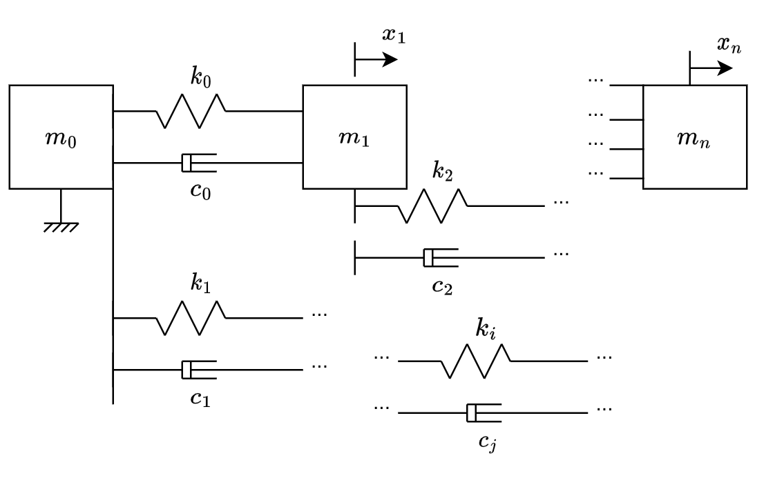
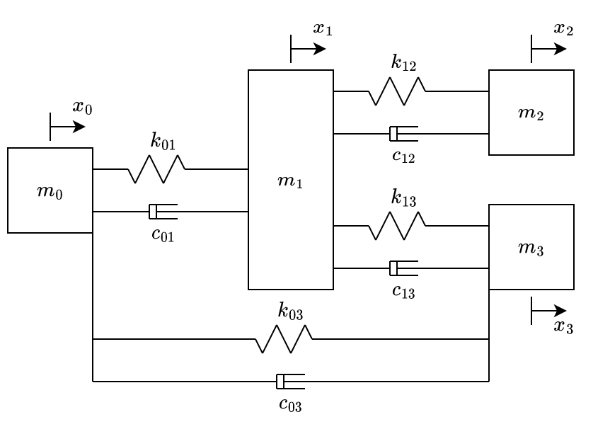
Consider a mechanical system comprized of ideal masses, ideal linear springs and ideal linear dampers, such as from fig. 2. (\(m_0\), \(m_1\), …,\(m_n\)) represent the masses, (\(k_0\), \(k_1\), …,\(k_i\)) represent the elastic constants of the springs and (\(c_0\), \(c_1\), …,\(c_j\)) represent the damping coefficient of the dampers. Note that \(m_0\) is fixed, but all the others have arbitrary initial displacement and velocities.
The optimization problem is stated as: Given the masses, the initial conditions (\(x_1(t=0)\), …,\(x_n(t=0)\), \(\dot{x_1}(t=0)\), …,\(\dot{x_n}(t=0)\)), the maximum and minimum values of each \(k_i\) and \(c_j\), and an impact duration \(T\), find (\(k_0\), …,\(k_i\), \(c_0\), …,\(c_j\)) that minimize \(\ddot{x_n}\) from \(t=0\) to \(t=T\).
6.3 Discrete element method
In order to explicitly integrate a mechanical system with respect to time, the ODE that describes the system is necessary. The discrete element method is a method to obtain the ODE for CMs.
6.3.1 Local Matrices
Fig. 3 shows the simplest system that contains ideal masses, springs and dampers. The spring has its natural/relaxed length when \(x_0=x_1=0\).
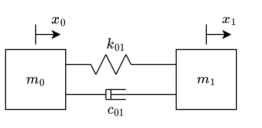
Considering that the elastic force \(F_k\) is linear with respect to the displacement (\(F_k = k \cdot x\)) and that the damping force \(F_c\) is linear with respect to the speed (\(F_x = c \cdot \dot{x}\)), from Newton’s second law we obtain eq. 1, in which \(\dot{x_i}\) and \(\ddot{x_i}\) represent the first and second time derivative of the displacement (with respect to the springs’ relaxed position) of the mass \(i\).
\[ \begin{bmatrix} -k_{01} & k_{01}\\ k_{01} & -k_{01} \end{bmatrix} \begin{bmatrix} x_0\\ x_1\\ \end{bmatrix} + \begin{bmatrix} -c_{01} & c_{01}\\ c_{01} & -c_{01} \end{bmatrix} \begin{bmatrix} \dot{x_0}\\ \dot{x_1}\\ \end{bmatrix} = \begin{bmatrix} m_0 & 0\\ 0 & m_1 \end{bmatrix} \begin{bmatrix} \ddot{x_0}\\ \ddot{x_1}\\ \end{bmatrix} \qquad{(1)}\]
Rewriting the above equation: \[ K_{l} \begin{bmatrix} x_0\\ x_1\\ \end{bmatrix} + C_{l} \begin{bmatrix} \dot{x_0}\\ \dot{x_1}\\ \end{bmatrix} = M_{l} \begin{bmatrix} \ddot{x_0}\\ \ddot{x_1}\\ \end{bmatrix} \qquad{(2)}\]
The matrices \(K_{l}\), \(C_{l}\) and \(M_{l}\) are termed, respectively, local stiffness matrix, local damping matrix and local mass matrix.
6.3.2 Assembling the global matrix
By adding another mass, spring and damper to fig. 3, we can obtain the system at fig. 4.
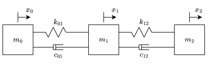
Equations of motion of system illustrated at fig. 4, also obtained by Newton’s second law, are:
\[ \begin{aligned} & \begin{bmatrix} -k_{01} & k_{01} & 0\\ k_{01} & -k_{01} {\color{blue}- k_{12}} & {\color{blue} k_{12}} \\ 0 & {\color{blue}k_{12}} & {\color{blue}-k_{12}} \\ \end{bmatrix} \begin{bmatrix} x_0\\ {\color{blue}x_1}\\ {\color{blue}x_2} \end{bmatrix} \\ & + \begin{bmatrix} -c_{01} & c_{01} & 0\\ c_{01} & -c_{01} {\color{blue}- c_{12}} & {\color{blue} c_{12}} \\ 0 & {\color{blue}c_{12}} & {\color{blue}-c_{12}} \\ \end{bmatrix} \begin{bmatrix} \dot{x_0}\\ {\color{blue}\dot{x_1}}\\ {\color{blue}\dot{x_2}} \end{bmatrix} = \\ & \begin{bmatrix} m_0 & 0 & 0\\ 0 & {\color{blue}m_1} & 0\\ 0 & 0 & {\color{blue}m_2}\\ \end{bmatrix} \begin{bmatrix} \ddot{x_0}\\ {\color{blue}\ddot{x_1}}\\ {\color{blue}\ddot{x_2}} \end{bmatrix} \end{aligned} \qquad{(3)}\]
By adding another mass, spring and damper connected to \(m_1\), we get the system at fig. 5.
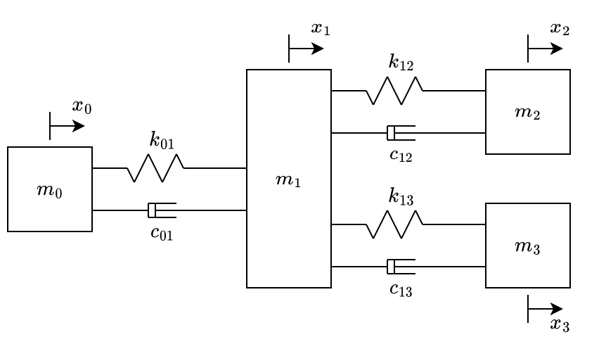
The equations of motion of the system illustrated at fig. 5 are:
\[ \begin{aligned} \begin{bmatrix} -k_{01} & k_{01} & 0& 0\\ k_{01} & -k_{01} - k_{12} {\color{blue}- k_{13}} & k_{12} & {\color{blue} k_{13}}\\ 0 & k_{12} & -k_{12} & 0\\ 0 & {\color{blue} k_{13}}& 0& {\color{blue} -k_{13}}\\ \end{bmatrix} \begin{bmatrix} x_0\\ {\color{blue}x_1}\\ x_2\\ {\color{blue}x_3} \end{bmatrix} + & \\ \begin{bmatrix} -c_{01} & c_{01} & 0& 0\\ c_{01} & -c_{01} - c_{12} {\color{blue}- c_{13}} & c_{12} & {\color{blue} c_{13}}\\ 0 & c_{12} & -c_{12} & 0\\ 0 & {\color{blue} c_{13}}& 0& {\color{blue} -c_{13}}\\ \end{bmatrix} \begin{bmatrix} \dot{x_0}\\ {\color{blue}\dot{x_1}}\\ \dot{x_2}\\ {\color{blue}\dot{x_3}} \end{bmatrix} =&\\ \begin{bmatrix} m_0 & 0 & 0 & 0 \\ 0 & {\color{blue}m_1} & 0 & 0 \\ 0 & 0 & m_2 & 0 \\ 0 & 0 & 0 & {\color{blue}m_3} \end{bmatrix} & \begin{bmatrix} \ddot{x_0}\\ {\color{blue}\ddot{x_1}}\\ \ddot{x_2}\\ {\color{blue}\ddot{x_3}} \end{bmatrix} \end{aligned} \qquad{(4)}\]
By adding just an extra spring and a damper connecting \(m_0\) and \(m_3\), we get the system at fig. 6.
The equations of motion of the system illustrated at fig. 6 are:
\[ \begin{aligned} \begin{bmatrix} -k_{01} {\color{blue}-k_{03}} & k_{01} & 0& {\color{blue}k_{03}}\\ k_{01} & -k_{01} - k_{12} - k_{13} & k_{12} & k_{13}\\ 0 & k_{12} & -k_{12} & 0\\ {\color{blue}k_{03}} & k_{13}& 0& -k_{13}{\color{blue}-k_{03}}\\ \end{bmatrix} \begin{bmatrix} {\color{blue}x_0}\\ x_1\\ x_2\\ {\color{blue}x_3} \end{bmatrix} + & \\ \begin{bmatrix} -c_{01} {\color{blue}-c_{03}} & c_{01} & 0& {\color{blue}c_{03}}\\ c_{01} & -c_{01} - c_{12} - c_{13} & c_{12} & c_{13}\\ 0 & c_{12} & -c_{12} & 0\\ {\color{blue}c_{03}} & c_{13}& 0& -c_{13}{\color{blue}-c_{03}}\\ \end{bmatrix} \begin{bmatrix} {\color{blue}\dot{x_0}}\\ \dot{x_1}\\ \dot{x_2}\\ {\color{blue}\dot{x_3}} \end{bmatrix} =&\\ \begin{bmatrix} {\color{blue}m_0} & 0 & 0 & 0 \\ 0 & m_1 & 0 & 0 \\ 0 & 0 & m_2 & 0 \\ 0 & 0 & 0 & {\color{blue}m_3} \end{bmatrix} & \begin{bmatrix} {\color{blue}\ddot{x_0}}\\ \ddot{x_1}\\ \ddot{x_2}\\ {\color{blue}\ddot{x_3}} \end{bmatrix} \end{aligned} \qquad{(5)}\]
By looking at eqns. 3-5, we can see that the equations of motion of the whole system are obtained by superposing the local matrices of each element, shown at eq. 1. The local matrices that are being added are highlighted in \(\textcolor{blue}{\text{blue}}\).
This is the same process done at the Finite Element Method (FEM) to assemble the global matrices from the elements’ local matrices. The reader can find in more detail at [9], [10].
6.4 Explicit Time Integration (ETI)
The Discrete Element Method can be use to obtain a CM’s ODE, i.e. the system’s state vector \(X\) and an expression \(\dot{X}(X)\) that calculates the state vector’s time derivative based on the current state. The ODE can then be integrated with an explicit method such as Forward Euler. Starting with the initial conditions, which are given, these methods recursively calculate the state of a system at a later time based on its state at a current time.
The output of the integration is the time response of the system, i.e. the displacement, velocity and acceleration of all the masses. This way, the maximum acceleration that each mass will experience - which is the loss function that is to be minimized with the COPs - can be obtained.
We can represent the state of the system with the state vector \(X\): \[ X = \begin{bmatrix} x_0\\ x_1\\ \vdots\\ x_n\\ \dot{x_0}\\ \dot{x_1}\\ \vdots\\ \dot{x_n} \end{bmatrix} \]
It’s time derivative is given by: \[ \dot{X} = \begin{bmatrix} \dot{x_0}\\ \dot{x_1}\\ \vdots\\ \dot{x_n}\\ \ddot{x_0}\\ \ddot{x_1}\\ \vdots\\ \ddot{x_n} \end{bmatrix} \]
Notice that the first half of \(\dot{X}\) is, simply, the second half of the \(X\). Hence, we just need to find expressions for the second derivatives of the displacements (\(\ddot{x_1}\), … , \(\ddot{x_n}\)).
After assembling the global matrices, we’ll be left with a matrix equation in the following form: \[ K \begin{bmatrix} x_0\\ x_1\\ \vdots\\ x_n \end{bmatrix} + C \begin{bmatrix} \dot{x_0}\\ \dot{x_1}\\ \vdots\\ \dot{x_n} \end{bmatrix} = M \begin{bmatrix} \ddot{x_0}\\ \ddot{x_1}\\ \vdots\\ \ddot{x_n} \end{bmatrix} \]
We can always multiply both sides by \(M^{-1}\), since \(M\) is a diagonal matrix with strictly positive numbers in the diagonal. This way, the system’s ODE is defined by the two following equations: \[ \begin{aligned} & X = \begin{bmatrix} x_0\\ x_1\\ \vdots\\ x_n\\ \dot{x_0}\\ \dot{x_1}\\ \vdots\\ \dot{x_n} \end{bmatrix} \quad\quad\text{,}\quad\quad \dot{X} = \begin{bmatrix} \dot{x_0}\\ \dot{x_1}\\ \vdots\\ \dot{x_n}\\ \ddot{x_0}\\ \ddot{x_1}\\ \vdots\\ \ddot{x_n} \end{bmatrix} \\\\ & \begin{bmatrix} \ddot{x_0}\\ \ddot{x_1}\\ \vdots\\ \ddot{x_n} \end{bmatrix} = M^{-1} \left( K \begin{bmatrix} x_0\\ x_1\\ \vdots\\ x_n \end{bmatrix} + C \begin{bmatrix} \dot{x_0}\\ \dot{x_1}\\ \vdots\\ \dot{x_n} \end{bmatrix} \right) \end{aligned} \qquad{(6)}\]
Note that inverting \(M\) is trivial, since it’s diagonal.
The initial conditions can then be applied directly at the \(\dot{X}\) vector. For fixed masses, for example, we just need to replace the appropriate element of \(\dot{X}\) with zero.
Example
Taking the system of fig. 3. Considering that the mass on the left is fixed and the one at the right starts with a positive initial displacement: \[ \begin{aligned} &m_0 \text{ is fixed} \\ &k_{01} = c_{01} = 1 \\ &m_1=1 \\ &x_0|_{t=0} = x_1|_{t=0} = 10 \\ &\dot{x_1}|_{t=0} = 0 \end{aligned} \qquad{(7)}\]
The state vector for this problem is: \[ X = \begin{bmatrix} x_0\\ x_1\\ \dot{x_0}\\ \dot{x_1} \end{bmatrix} \]
By assembling the system’s global matrices (which was already done at eq. 1), from eq. 6 we have: \[ \begin{bmatrix} \ddot{x_0}\\ \ddot{x_1}\\ \end{bmatrix} = \begin{bmatrix} 1/m_0 & 0\\ 0 & 1/m_1 \end{bmatrix} \left( \begin{bmatrix} -k_{01} & k_{01}\\ k_{01} & -k_{01} \end{bmatrix} \begin{bmatrix} x_0\\ x_1\\ \end{bmatrix} + \begin{bmatrix} -c_{01} & c_{01}\\ c_{01} & -c_{01} \end{bmatrix} \begin{bmatrix} \dot{x_0}\\ \dot{x_1}\\ \end{bmatrix} \right) \]
Replacing the values from eq. 7: \[ \begin{bmatrix} \ddot{x_0}\\ \ddot{x_1}\\ \end{bmatrix} = \begin{bmatrix} 1/m_0& 0\\ 0 & 1 \end{bmatrix} \left( \begin{bmatrix} -1 & 1\\ 1 & -1 \end{bmatrix} \begin{bmatrix} x_0\\ x_1\\ \end{bmatrix} + \begin{bmatrix} -1 & 1\\ 1 & -1 \end{bmatrix} \begin{bmatrix} \dot{x_0}\\ \dot{x_1}\\ \end{bmatrix} \right) \]
\[ \begin{bmatrix} \ddot{x_0}\\ \ddot{x_1}\\ \end{bmatrix} = \begin{bmatrix} 1/m_0(-x_0+x_1-\dot{x_0}+\dot{x_1})\\ x_0-x_1+\dot{x_0}-\dot{x_1} \end{bmatrix} \]
Since we considered \(m_0\) to be fixed, we replace the expression of \(\ddot{x_0}\) with \(0\):
\[ \begin{bmatrix} \ddot{x_0}\\ \ddot{x_1}\\ \end{bmatrix} = \begin{bmatrix} 0\\ x_0-x_1+\dot{x_0}-\dot{x_1} \end{bmatrix} \]
Thus, the ODE is defined as: \[ X = \begin{bmatrix} x_0\\ x_1\\ \dot{x_0}\\ \dot{x_1} \end{bmatrix} \quad\quad\text{ and }\quad\quad \dot{X} = \begin{bmatrix} \dot{x_0}\\ \dot{x_1}\\ 0\\ x_0-x_1+\dot{x_0}-\dot{x_1} \end{bmatrix} \]
If the ODE were to be integrated with a simple Forward Euler using a \(0.1\) time-step, the first time-step would be:
- t = 0 (initial values taken from eq. 7)
\[ X|_{t=0} = \begin{bmatrix} 0\\ 10\\ 0\\ 0 \end{bmatrix} \]
\[ \dot{X} = \begin{bmatrix} \dot{x_0}\\ \dot{x_1}\\ 0\\ x_0-x_1+\dot{x_0}-\dot{x_1} \end{bmatrix} \rightarrow \dot{X}|_{t_0} = \begin{bmatrix} 0\\ 0\\ 0\\ -10 \end{bmatrix} \]
- t = 0.1
\[ X|_{t=0.1} = X|_{t=0} + 0.1 \cdot \dot{X}|_{t_0} = \begin{bmatrix} 0\\ 10\\ 0\\ 0 \end{bmatrix} + 0.1 \begin{bmatrix} 0\\ 0\\ 0\\ -10 \end{bmatrix} \]
\[ X|_{t=0.1} = \begin{bmatrix} 0\\ 10\\ 0\\ -1 \end{bmatrix} \]
6.4.1 Software
See sec. 4.7 for how we implemented explicit time integration of CMs.
6.5 Genetic Algorithm
The genetic algorithm is an optimization and search technique based on the principles of genetics and natural selection [11]. Some of its advantages, when compared to gradient base methods, are [11]:
- Doesn’t require derivative information
- Simultaneously searches from a wide sampling of the cost surface
- Deals with a large number of variables
- Is well suited for parallel computers
- Optimizes variables with extremely complex cost surfaces (they can jump out of local minima)
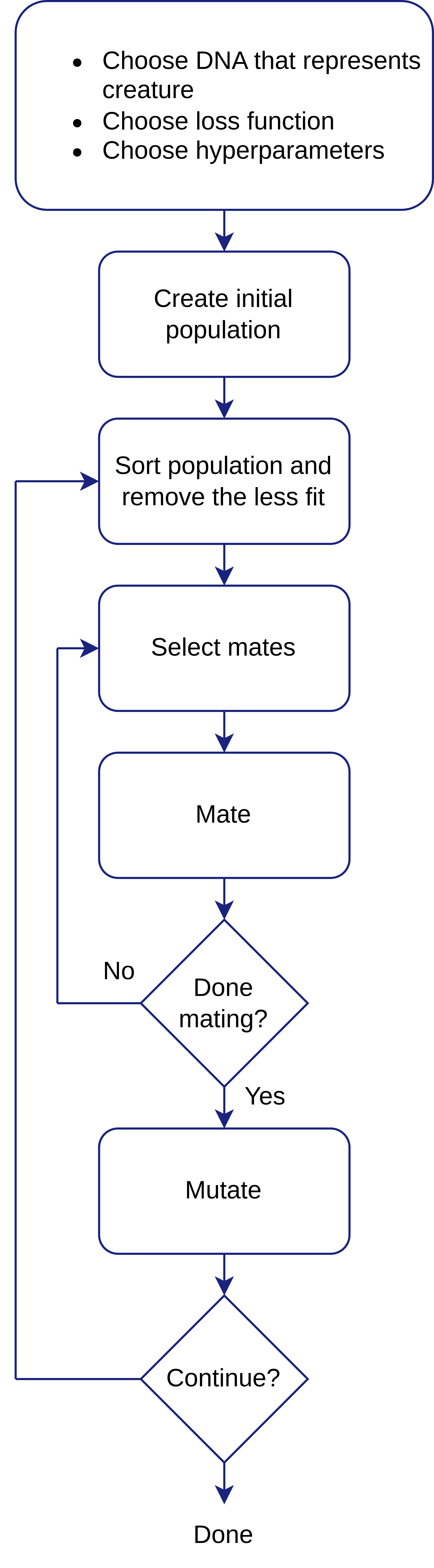
There’s no single recipe for success of GAs. Many details vary slightly between implementations - such as the use of elitism the criteria for selecting mates and the breeding process - but fig. 7 illustrates a high level overview of all components of the Genetic Algorithm as we implemented it. In this section, the components, as we implemented them in our code, are briefly explained and an example involving all the steps is presented.
The main sources this section is based on are [11]–[13].
The Evolve (/software/evolution.tcc) method is the top-level-method which executes the GA optimization. It basically performs the initial sorting of the population, checks for convergence and successively calls the step (/software/evolution.tcc) method, which performs one iteration of optimization of the population.
6.5.1 GA steps
Choose DNA that represents creature
Given GA’s biological inspirations, possible solutions to the problem at hand are often referred to as creatures. For example, if we use GA to find the minimum value of a function \(f(x,y)\), \(\{x,y\}\) pairs, such as \(\{0,0\}\), \(\{1,0\}\), can be thought of as creatures.
In GA, we must define what the DNA of our problem’s creatures is. For real-encoded - also known as continuous - GA, which is the one we’re interested in, the DNA is simply a vector of real numbers. So for the problem we mentioned above in which creatures are described by pairs of \(x\) and \(y\), we could choose that the creatures’ DNA is simply a vector in which the first element is the value of \(x\) and the second is the value of \(y\). Note that we could also choose the other order. Thus, it’s up to the user to choose how to model the problem.
Another example: let’s say the problem at hand is that of finding values for the springs and dampers of the system illustrated at fig. 6 which minimize the maximum acceleration \(m_3\) experiences if the whole system is traveling with a constant speed towards the left and hits an immovable object. A creature in this problem is a set of values of springs’ and dampers’ constants. We can choose, for example, that the DNA that represents a creature is the vector \([k_{01},c_{01},k_{12},c_{12},k_{13},c_{13},k_{03},c_{03}]\).
Note that when defining a DNA, we must also define what our domain is, i.e. in what range each DNA member must be in.
Choose fitness function
In this step, we need to define a function that measures how good each creature is, so that we can sort the population by goodness. This function takes a creature - or more specifically its DNA - as input, and returns a real value, i.e. a scalar.
Choose hyperparameters
Hyperparameters are top-level parameters we choose for the optimization algorithm itself. In this case, we must choose:
- Population size
- Population survival rate
- Mutation rate
The meaning of these values will become clearer in the following example.
Create initial population
At this step, we initialize a population of random creatures.
Sort population and remove the less fit
We begin this step by calculating the fitness function of each creature. Then, we sort the population by descending fitness function value. A portion, determined by the population survival rate hyperparameter, of the less fit population (the creatures with the lowest fitness function values) is then removed from the population. This stage is equivalent to the survival of the fittest in the evolutionary process.
Select mates
In this step, creatures which will mate to create offspring that will replace the creatures which were removed at the last stage must be selected.
There are many different approaches to doing this. Some of them are highlighted at [12], [13]. In our code, we used what’s known as Biased Roulette Wheel Selection. In this process, two creatures are selected randomly, but the probability of a creature being selected is proportional to how high their fitness function value is. For more detail on how this done, we suggest one to see getParents (/software/evolution.tcc) implementation.
Mate
In this step, two creatures which were selected in the previous step - the parents - mate to create two new creatures : the children. Again, there are also many different techniques for this process (see [11]). We implemented what’s known as Radcliff blending method [11], which is as follows:
Let \(\text{D}_{p0}\) and \(\text{D}_{p1}\) be the DNA of the parents, and \(\text{D}_{c0}\) and \(\text{D}_{c1}\) be the DNA of the children which will be created. \(\text{D}_{x}[i]\) corresponds to the \(i\)-th position of \(x\)’s DNA.
For every valid index \(i\):
- A random variable \(\beta\) in the range \([0, 1]\) is created.
- \(\text{D}_{c0}[i] = \beta \text{D}_{p0}[i] + (1-\beta \text{D}_{p1}[i])\)
- \(\text{D}_{c1}[i] = \beta \text{D}_{p1}[i] + (1-\beta \text{D}_{p0}[i])\)
This logic is implemented at the Mate (/software/creature.cc) method.
The two created children fill the gaps in the population of the less fit creatures which were removed at the Sort population and remove the less fit step. If there’s only room left in the population for one creature, one of them is just discarded.
Done mating?
If the current population size is still smaller than the population size hyperparameter, we continue with the mating process.
Mutate
At this stage, we apply random mutations to only the children which were created (which is called elitism). Elitism guarantees that the fittest creatures from one iteration of the algorithm are either just as fit or less fit than the fittest ones from the next iteration of the algorithm.
We implemented uniform random mutation, which means that to perform a mutation we do the following:
- Pick a random child which was created
- Choose a random position of the DNA
- Let \(a\) and \(b\) be the minimum and maximum value acceptable for this position at the DNA. Replace the value at that position with a random number in the interval \([a,b]\)
The number of mutations we perform is determined by the mutation rate hyperparameter. For a mutation rate \(m\), population size \(p\), survival rate \(s\) and the creatures’ DNA size \(d\), the number of mutations that will be performed is given by \(m \cdot p(1-s)d\).
The idea behind this is that we allow us only to mutate the children. Thus, there are \(p(1-s)\) creatures that can suffer mutation. Each has \(d\) DNA slots. Hence, there are \(p(1-s)d\) DNA slots we can mutate. We multiply that by the mutation rate, which is a number between \(0\) and \(1\), and get the number of DNA slots we’ll mutate.
This logic is implemented at the mutate (/software/evolution.tcc) method.
Continue?
Whenever we reach this stage, we consider to have finished a generation. We now choose to stop if the algorithm has converged, i.e. the value of the fitness function of the fittest creatures is practically the same it was on the previous generation, or if too many generations have been tried but the algorithm still hasn’t converged.
Summary
6.5.2 GA steps illustrative example
Suppose we want to find the value of \(\{x,y\}\) in the region \(x \in [-2,2]\) and \(y \in [-2,2]\) that minimizes the function
\[ f(x,y) = x^2 + y^2 + 2x + y \]
Choose DNA that represents creature
The creatures of this problem are pairs \(\{x,y\}\), so we can choose the DNA of each creature to be the vector \([x,y]\)
Choose fitness function
Instead of defining a fitness function, in this case we’ll define a
loss function for simplicity. The only difference between
the two is that low values of loss indicate good solutions,
whereas high values of fitness indicate good solutions.
Since we want to minimize \(f\), the loss function for a creature with DNA \([x_c,y_c]\) can simply be:
\[ loss(x_c,y_c) = x_c^2 + y_c^2 + 2x_c + y_c \]
The lowest the value of loss, the better the candidate
solution is.
Choose hyperparameters
Since this is just an illustrative example, we chose:
- Population size \(=4\)
- Population survival rate \(=0.5=50\%\)
- Mutation rate \(=0.25\)
Note that outside illustrative examples the population sizes are usually much higher and the mutation rates are usually much smaller.
Create initial population
By picking random numbers between \(-2\) and \(2\) we obtained the following population:
\[ [[0.4, 0.16], [-0.9, 0.2], [-0.2, 0.2], [0.1, -0.1]] \qquad{(8)}\]
Sort population and remove the less fit
The loss function calculated for each creature at eq. 8 has the following values:
\[ [1.1456,-0.75,-0.12,0.12] \]
Thus, the sorted population (from smallest to largest loss) becomes: \[ [[-0.9, 0.2], [-0.2, 0.2], [0.1, -0.1], [0.4, 0.16]] \]
With a survival rate of \(50\%\), we get: \[ [[-0.9, 0.2], [-0.2, 0.2]] \]
Select mates
In this case, since there are only 2 creatures, we have no choice but to select them as parents. However, the roulette wheel algorithm, which is implemented at the getParents (/software/evolution.tcc) method would be as follows:
First we transform the loss value so that they’re strictly positive and high values indicate goodness. We can do that by adding \(1.75\) to all the values, and then taking the inverse of the value:
\[ [-0.75,-0.12] \rightarrow [1,1.63] \rightarrow [1,0.61] \]
We then normalize the values: \[ [1,0.61] \rightarrow [0.62, 0.38] \]
Lastly, we accumulate the values, so that they’re always growing. \[ [0.62, 0.38] \rightarrow [0.62, 1] \]
Now, to select a parent we create a random number between \(0\) and \(1\). If the random number is \(<=0.62\), we select the first creature as parent. Else, we select the second. We then pick another random number to choose the other parent. In cases when the same parent is selected twice by chance, we take the next parent.
Mate
For the random number \(\beta = 0.1\), the DNAs of the children would be:
\[ \begin{aligned} &[0.1\cdot(-0.9) + (1-0.1)\cdot(-0.2), 0.1\cdot(0.2) + (1-0.1)\cdot(0.2)] = [-0.27, 0.2]\\ &[0.1\cdot(-0.2) + (1-0.1)\cdot(-0.9), 0.1\cdot(0.2) + (1-0.1)\cdot(0.2)] = [-0.83, 0.2] \end{aligned} \]
After adding them to the population we get:
\[ [[-0.9, 0.2], [-0.2, 0.2], [-0.27, 0.2], [-0.83, 0.2]] \]
Mutate
Two children were created. They each have 2 DNA slots. Thus, there are, in total, 4 DNA slots which can suffer mutation. A mutation rate of 25% means we’ll mutate 1 DNA slot.
To perform the mutations we first pick a random child. Then, we pick a random DNA index, and replace the value there with a random one between \(-2\) and \(2\).
For example, with the following events:
- First child was randomly selected
- Second DNA index was randomly selected
- 0.7 was randomly selected in the range [-2,2]
The final population becomes:
\[ [[-0.9, 0.2], [-0.2, 0.2], [-0.27, 0.7], [-0.83, 0.2]] \]
6.5.3 Software
See sec. 4.8 for how we implemented GA optimization of CMs to solve COPs.
6.6 ML-Model-Based-Genetic-Algorithm for Mechanical Optimization
[1], [3], [4] are among the main sources of inspiration for this work. They all studied the use of metamodels in conjunction with Genetic Algorithm for optimization of materials/solid structures in a vast design space, and were very successful. The metamodels used provided a very significant improvement in performance, and the obtained solutions were very efficient. [5] studied using metamodels to predict the behavior of highly non-linear 3D lattice structure.
All the studies mentioned above had to go through a very computationally expensive process of generating labeled data and training the metamodels.
[6], [7] have studied PIMs, which can be trained without labeled data. These models make it possible to bypass the stage of training data generation. This led us to wonder if PIMs might be the ideal metamodels for metamodel-based-GAs. However, we didn’t find in the literature studies which combine PIMs with GAs.
6.7 Physics-Informed Machine Learning
We start by explaining the basic concepts of Machine Learning, and then show how the same ideas, with some small modifications, are applied to solve problems which are described by partial differential equations.
The problems we choose to solve are very simple, but they’re great for illustrating the basic principles.
6.7.1 Introduction to Machine Learning
Consider the data in tbl. 2.
| \(t\) | \(y\) |
|---|---|
| 10 | 1.0 |
| 20 | 2.1 |
| 30 | 3.0 |
Let’s say we want to model the relationship between \(x\) and \(y\) in a linear model in the form \(\bar{y}(t) = at + b\), where \(a\) and \(b\) are real constants. This would allow us to approximate the values of \(y\) for values of \(x\) other than the ones we have in our dataset. Note that the model we choose is arbitrary. We could pick any other much more complicated model of higher order, but we’ll stick to this linear one because the principles are the same.
For example, a possible model would be \(\bar{y}(t) = 2t + 5\). That would, however, be terrible to model our data, as the difference between the model and the real values are very big. Hence, we want to find values of \(a\) and \(b\) that cause our model to make predictions close to the real values. Ideally, we’d want \(\bar{y}(t_i) = y_i\) for all \(t_i\) from tbl. 2. An expression that we can use to measure how well our model fits to the data is to calculate the sum of the square of the residues:
\[ R = \sum_{t_i} (\bar{y}(t_i)-y_i)^2 = (\bar{y}(10)-y_0)^2 + (\bar{y}(20)-y_1)^2 + (\bar{y}(30)-y_2)^2 \]
We take the square of the residues so that residues of opposite signs do not cancel each other out. This is equivalent to taking the absolute value of the residue, but much more mathematically convenient.
Replacing the definition of \(\bar{y}\) and the \(y_i\) values from tbl. 2:
\[ R = (10a + b -1)^2 + (20a + b -2.1)^2 + (30a + b - 3.0)^2 \]
From now on, our problem becomes finding values of \(a\) and \(b\) that minimize \(R\).
We can find those values with the gradient descent method. Since we can calculate the derivatives of \(R\) with respect to \(a\) and \(b\), we can also calculate its gradient, which can be thought of as a vector in the \(a,b\) plane which points in the direction in which \(R\) increases the most:
\[ \nabla R = \begin{bmatrix} \frac{\partial R}{\partial a} \\ \frac{\partial R}{\partial b} \end{bmatrix} = \begin{bmatrix} 2800 a + 120 b - 284 \\ 120 a + 6 b - 12.2 \end{bmatrix} \]
The basic idea in the gradient descent method is to start with random \(a\) and \(b\) values, and make successive steps in the opposite direction of the gradient. The code listing bellow, written in python, exemplifies how gradient descent can be performed:
def grad(a,b):
    return (2800*a + 120*b - 284, 120*a + 6*b - 12.2)

a = 1
b = 1
l = 0.00001
for i in range (10000000):
    g = grad(a,b)
    a = a - l*g[0]
    b = b - l*g[1]

print(a,b)
The listing above outputs \(a = 0.0999\) and \(b = 0.0333\), which is, up to numerical precision, exactly like the analytical solution.
Thus, we find that our model has the following expression, which yields results very close to tbl. 2:
\[ \bar{y}(t) = 0.099t + 0.033 \]
Since we’re just using an example to illustrate the principles of ML, we chose a very simple model, with a single input, and very few data points. However, the general workflow is the same for real like applications:
- Define a model
- Choose loss function that has the model’s parameters (in our example those were just \(a\) and \(b\)) as arguments, and measures, using the data we have available, how well our model’s predictions match the expected outputs
- Minimize the loss function to find the optimal parameters for the model
6.7.2 Introduction to Physics-Informed Machine Learning
What if instead of having values for \(t\) and \(y\), we had an expression for \(\ddot{y}\), the second time derivative of \(y\)? For example: Consider a ball that is thrown upwards with an initial velocity of \(10\)m/s. With \(y\) as the height of the ball and considering \(10\)m/s\(^2\) as gravity’s acceleration, the physical equation that governs this motion is:
\[ \ddot{y} = -10 \qquad{(9)}\]
We can solve this problem in the same way as we did the previous one by just doing some modifications. First, we must define the model we want to use to approximate \(y\). Let \(\bar{y}(t)\) be the model, given by:
\[ \bar{y}(t) = a\cdot t^2 + b\cdot t + c \qquad{(10)}\]
We chose this because we can then compare the solution we obtain with the analytical solution \(y(t) = -5t^2+10t\).
The next step is to define a loss function. In this case, we only have value for \(y\) at \(t=0\) (considering that the ball starts at position \(y=0\)). We also have value for the first derivative of \(y\) at \(t=0\), which is the initial speed. For all other instants of time, we only know the second derivative of \(y\) from eq. 9. To write a loss function, we can first define multiple values of \(t\) which are of interest. Then, the loss function can calculate the residues for \(y\) and \(\dot{y}\) at \(t=0\), and for \(\ddot{y}\) for all other time instants:
Let \(t = [0, 0.1, 0.2, ... , 1.0]\). The loss function \(R\) is given by:
\[ R = (\bar{y}(0)-y|_{t=0})^2 + (\dot{\bar{y}}(0)-\dot{y}|_{t=0})^2 + \sum_{i=0}^{10} (\ddot{\bar{y}}(0.1 i)-\ddot{y})^2 \]
Note that we can use this technique because we chose what we want the model \(\bar{y}\) to be like; so we can easily calculate its time derivative. Replacing \(\bar{y}(t)\) with its definition from eq. 10, \(y|_{t=0}\) with \(0\) and \(\dot{y}|_{t=0}\) with \(10\) (the initial velocity), we get:
\[ R = (c-0)^2 + (b-10)^2 + \sum_{i=0}^{10} (2a+10)^2 \]
All we’re left to do now is to find the values of \(a\), \(b\) and \(c\) that minimize \(R\). The gradient of R is given by: \[ \nabla R = \begin{bmatrix} \sum_{i=0}^{10} 4(2a+10) \\ 2(b-10) \\ 2c \end{bmatrix} \]
A simple python script that can be used to perform gradient descent is the following:
nT = 10

def grad(a,b,c):
    ga = 0
    for i in range (nT+1):
        t = 1/nT*i
        ga += 4*(2*a+10)

    gb = 2*(b-10)

    gc = 2*c

    return (ga,gb,gc)

a = 0
b = 0
c = 0
l = 0.0001
for i in range (100000):
    g = grad(a,b,c)
    a = a - l*g[0]
    b = b - l*g[1]
    c = c - l*g[2]
    print(a,b,c)
The output of the above script is -4.9999 9.9999 0.0
which is, up to numerical precision, exactly like the analytical
solution.
[14] is an excellent source that covers, in great depth and breadth, the fundamentals of physics based models and the usage of more sophisticated models such as deep neural networks.
7 Methods
7.1 Overview
The method used to achieve the objectives listed at sec. 2 was to implement a library that is capable of:
- E-GA evaluates candidate solutions using explicit time integration (see sec. 3.4).
- P-GA evaluates candidate solutions using PIMs which describe the position of each mass as a function of time and of the values of the springs and dampers of the system. The PIMs used are linear regression models (see sec. 4.2).
Using this library, we performed a few COP case studies using both P-GA and E-GA. The performance and the result of each algorithm were then compared. Performance of each algorithm was measured by the total processing time needed for the optimization to finish. We compared the results by comparing the maximum acceleration the mass would experience with the optimal solution found by the algorithm.
7.2 Polynomial Models
The PIMs we used in this work are based on linear regression models. The expression of the models is defined by the number of springs/dampers of the CM we’re trying to optimized, and by the order of the polynomials. The order defines the highest order of the monomials.
For an order \(h\), the models have the following expression:
\[ \begin{aligned} p_h(t, k_1, k_2, ... , k_i, c_1, c_2,..., c_j) = \sum_{\lambda=0}^{\lambda=h} a_\mu t^\lambda + &\sum_{Z} a_\mu t^\eta k_1^{\gamma_1} k_2^{\gamma_2} ... k_i^{\gamma_i} c_1^{\omega_1} c_2^{\omega_2} ... c_j^{\omega_j}\\ &Z = \{1 <= \eta < h, (\gamma_i = 0 \text{ OR } \gamma_i = 1),\\ &(\omega_j = 0 \text{ OR } \omega_j = 1),\\ &{\textstyle(\sum \gamma_i + \sum \omega_j = 1)}\} \end{aligned} \qquad{(11)}\]
In plain english, that means that the polynomial is a linear combination of:
- All the powers of \(t\) from \(0\) to \(h\)
- Cross product of \([t^{h-1}, ..., t^2, t]\) and \([k_1, ..., k_i, c_1, ..., c_j]\)
For example, let’s consider a CM with 2 springs and 1 damper. Following are the expression that the models would take:
\[ p_0(t, k_1, k_2, c_1) = a_0 \]
\[ p_1(t, k_1, k_2, c_1) = a_0 + a_1t \]
\[ p_2(t, k_1, k_2, c_1) = a_0 + a_1t + a_2t^2 + a_3tk_1 + a_4tk_2 + a_5tc_1 \]
\[ p_3(t, k_1, k_2, c_1) = a_0 + a_1t + a_2t^2 + a_3t^3 +a_4t^2k_1 + a_5t^2k_2 + a_6t^2c_1 +a_7tk_1 + a_8tk_2 + a_9tc_1 \]
7.2.1 Reasoning behind the models’ architecture
The goal of this project was not to determine optimal model to represent the dynamic response of CMs; but rather just to analyze the P-GA approach as a whole.
The models defined by eq. 11 are convenient for many reasons:
Their gradients are easy to compute since they’re are linear.
For a given problem, the whole model architecture is defined by a single parameter (the order) of the models. This makes it super easy to increase/decrease the model complexity when needed.
Implementing differentiation and linear combinations of polynomial models is relatively easy to implement when compared to other models such as Neural Networks.
Note that the architecture of the models have a significantly strong assumption behind them: the largest order of t is always larger than the order of the other input variables (\(k_i\) and \(c_j\)). This characteristic is very much by design, because we know that the dynamic response of the CMs are usually not linear with respect to time. Still, the training of the models should be able to identify which monomials are more significant to model the systems.
Of course, an immediate opportunity of further research is to use different models and analyze how that changes the performance of P-GAs.
7.2.2 Automatic differentiation and linear combination
As it is thoroughly described in sec. 4.3, differentiating the models with respect to time and linearly combining them are two tasks that are required to build the loss function used to train the models.
As can be seen in /software/polynomial.cc, the classes implemented for representation/manipulation of polynomial models support automatic differentiation and the operators of polynomial instances Poly and Polys (/software/polynomial.cc) have been implemented so that they can be linearly combined even through matrix multiplications (see this test for example).
Side note
The /software/polynomial.cc implementation is one of the intermediary tasks of this project the author found the most challenging and interesting.
7.2.3 Software
/software/polynomial.h contains all the code related to the polynomial models. The Poly (/software/polynomial.h) class defines a single instance of a polynomial, and the Polys (/software/polynomial.h) class handles the linear combination of Poly instances.
As usual, /software/polynomial_test.cc contains tests which serve as documentation and usage examples.
7.3 Physics-Informed Machine Learning Models (PIMs)
7.3.1 Architecture of the models
As seen in sec. 3.7, Physics-Informed Machine Learning Models are trained so that they approximate the solution to a differential equation. In this work, we’re dealing not with one, but with a system of differential equations that describe the COP.
Consider an arbitrary COP of \(n\) masses. As seen in sec. 3.4, the \(n\) equations that describe the system, as obtained with the Discrete element method, have the following form:
\[ \begin{bmatrix} \ddot{x_0}\\ \ddot{x_1}\\ \vdots\\ \ddot{x_n} \end{bmatrix} = M^{-1} \left( K \begin{bmatrix} x_0\\ x_1\\ \vdots\\ x_n \end{bmatrix} + C \begin{bmatrix} \dot{x_0}\\ \dot{x_1}\\ \vdots\\ \dot{x_n} \end{bmatrix} \right) \qquad{(12)}\]
To use Physics-Informed Machine Learning Models for this problem, our approach was to have one model per mass that approximates the displacement (\(x_n\)) of each mass as a function of time (\(t\)) and of the constants of the springs and dampers (\(k_0, \cdots,k_i, c_0, \cdots,c_j\)). I.e. for a system of \(n\) masses, \(i\) springs and \(j\) dampers, we defined the polynomial models \(P_0(t, k_0, \cdots,k_i, c_0, \cdots,c_j), \cdots, P_n(t, k_0, \cdots,k_i, c_0, \cdots,c_j)\) so that \(P_0\) models \(x_0\), \(P_1\) models \(x_1\), etc.
Note that the models can easily be differentiated with respect to time so that we can obtain the velocity and acceleration of each mass. The order of the polynomials was a hyperparameter chosen for the experiments (see sec. 4.9 for more details).
7.3.2 Time discretization
Given that the time responses of the CMs are usually very non-linear with respect to time (see fig. 8 for example), using a model that describes the displacement of a mass for the whole duration of the impact would not be efficient. The model would need to have a very high order, which can make the training very slow.
To solve that, the approach we took was to discretize the time into multiple “buckets”. TimeDiscretization is defined as the number of buckets into which the total time of interest is split. Let’s say we want models that describe a COP from \(t=0\) to \(t=T\). Instead of having a set of models (one for each mass) that describes the displacement of each mass as a function of time from \(t=0\) to \(t=T\), we created a set of models (one for each mass) that describe the displacement of the masses from \(t=0\) to \(t=T_0\), then another set of models for \(t=T_0\) to \(t=T_1\), and so on until a set of models for \(t=T_i\) to \(t=T\). TimeDiscretization is a hyperparameter chosen for the experiments (see sec. 4.9 for more details).
To train those models, we start by training the first set of models - they describe the displacement of the masses from \(t=0\) to \(t=T_0\). Let’s call these the \(t_0\) models. The initial conditions (the displacement and velocity of each mass) are given by the COP statement. Then, to train the next set of models - the \(t_1\) models - we used the \(t_0\) models to find the conditions (displacement and velocity of each mass) at \(t=T_0\). These conditions are considered initial conditions for the next set of models. This process continues until all the \(t_i\) models are trained. At the end of this process, we have a set of models for each “time bucket”. See Pimodels::Train (/software/pimodel.cc) for more detail.
Note that the models have as input not only the time, but also the values of the springs and dampers. When using a “previous” set of models to determine the initial conditions to train the “next” set of models, we choose the intermediary values for the springs and dampers. I.e. for every spring/damper that can have values from \(a\) to \(b\), we used \((a+b)/2\) to evaluate the models.
7.3.3 Normalization
Normalizing the inputs to the models can yield faster training [15, p. 365]. Thus, the input to all
models were the normalized values from 0 to 1.
For the springs, 0 corresponded to minimum possible value
of the springs elastic constant and 1 to the maximum. The
analogous was used for the dampers. For time, 0
corresponded to the start of the impact and 1 to the end of
the impact (t=T). A linear normalization was used.
7.3.4 Training: Minimizing the loss function
As described in sec. 4.3.2, the total time of the COP is discretized and, progressively, one set of models is trained for each “time bucket”.
Initially, all the models are created with all the coefficients equal to zero; i.e. all the polynomial coefficients are 0. They are then trained, with Stochastic Gradient Descent [15, p. 184], to minimize a loss function. Following the usual formulation of Physics Informed Machine learning [14], the loss function is composed of 3 parts:
\(L_{x}\): Initial displacement loss
\(L_{\dot{x}}\): Initial velocity loss
\(L_{\ddot{x}}\): Physics loss
\(L_{x}\) measures how well the models estimate the initial displacement of the masses. \(L_{\dot{x}}\) measures how well the models estimate the initial velocity of the masses. \(L_{\ddot{x}}\) measures how well the models obey the physics, i.e. how well the fit the COP’s ODE (eq. 12).
For the following text, consider that \(s\):
\[ s={k_0}_{norm}, ...,{k_i}_{norm}, {c_0}_{norm}, ...,{c_j}_{norm} \qquad{(13)}\]
represents a set of springs and dampers that define a solution to a COP. The \(_{norm}\) subscript indicates that the values are normalized considering the maximum and minimum possible values of each spring and damper (see sec. 4.3.3). As an example, let’s consider a COP comprized of two masses connected by a spring of elastic constant \(k_0\) and a damper with damping coefficient \(c_0\). The spring can have values from \(10\) to \(20\), and the damper can have values from \(50\) to \(100\). \(s=\{0, 0.5\}\) represents a system with \(k_0 = 10\) and \(c_0 = 75\).
In our chosen approach, we want the models to not only be a function of time, but also of the system’s parameters (the springs and the dampers). Thus, we want the minimization of the losses to force the models to work well for multiple values of springs and dampers. We achieved that by computing the losses for multiple possible values of the springs and dampers as follows:
We start by defining a InitialConditionsTrainingSize. Let’s call that \(\alpha\) for now. We define a random set \(S\) of size \(\alpha\) that contains random values of \(s\) (see eq. 13):
\[ S = \{s_1, s_2, ... , s_{\alpha} \} \]
For a COP of \(n\) masses, let \(P_i\) indicate the model of the mass \(i\) (see sec. 4.3.1), \(L_{x}\) is then defined as:
\[ L_{x} = \sum_{i=1}^{n}\sum_{j=1}^{\alpha} (P_i(t = 0, s_j) - x_i|_{t=0})^2 \qquad{(14)}\]
In plain english, that equation is read as: Sum of the squared error of the model’s predicted displacement and the actual displacement at \(t=0\), for all the masses using all the random values of springs and dampers we randomly picked.
Note that the \(x_i|_{t=0}\) are the initial conditions of each mass, which are part of the COP definition.
The definition of \(L_{\dot{x}}\) is analogous, but for the initial velocities:
\[ L_{\dot{x}} = \sum_{i=1}^{n}\sum_{j=1}^{\alpha} (\dot{P_i}(t = 0, s_j) - \dot{x_i}|_{t=0})^2 \qquad{(15)}\]
Just note that \(\dot{P_i}\) is the derivative of the model with respect to the unnormalized time. See sec. 4.3.4.1 for more details.
eq. 12 is the ODE that the \(\ddot{x}_i\) must satisfy. This equation provides all the accelerations as a function of the springs, dampers, and of the displacement and velocities of all masses:
\[ \ddot{x_i} = F_i(x_0, x_1, \cdots, x_n, \dot{x_0}, \dot{x_1}, \cdots, \dot{x_i}, k_0, k_1, \cdots,c_0, c_1, \cdots) \qquad{(16)}\]
We want the models to fit eq. 16 not only for \(t=0\), but for all the interval of the COP. Consider that \(s_t\):
\[ s_t = t_{norm}, {k_0}_{norm}, ...,{k_i}_{norm}, {c_0}_{norm}, ...,{c_j}_{norm} \qquad{(17)}\]
represents a set of springs and dampers that define a solution to a COP and a time from 0 to 1. This is basically the same definition of eq. 13, but with time also as an argument. Similarly to how we built the other losses, we must define a PhysicsTrainingSize. Let’s call that \(\zeta\) for now. We define a set \(S_{t}\) of size \(\zeta\) that contains random values of \(s_t\) (see eq. 17):
\[ S_{t} = \{{s_t}_1, ... , {s_t}_{\zeta} \} \]
The physics loss function is then defined as:
\[ L_{\ddot{x}} = \sum_{i=1}^{n}\sum_{j=1}^{\zeta} (\ddot{P_i}({s_t}_j) - F_i( P_0({s_t}_j), P_1({s_t}_j), \cdots, \dot{P_0}({s_t}_j), \dot{P_1}({s_t}_j), \cdots, {s_t}_j ))^2 \qquad{(18)}\]
That equation is basically the sum of the errors of the second derivative of the model and what that second derivative should be according to the system’s ODE. Since the ODE expects the displacements and velocities of all the masses, we use the models themselves as estimators for those.
The total loss that we want to minimize is simply the sum of all losses:
\[ L = L_x + L_{\dot{x}} + L_{\ddot{x}} \qquad{(19)}\]
7.3.4.1 Change of variables for the time derivatives
The first element of the residue from eq. 18 - \(\ddot{P_i}({s_t}_j)\) - is a second derivative of the model with respect to time. As explained in sec. 4.3.3, the input of the model is not the actual time but rather the normalized time (from 0 to 1). To clearly distinguish those two, in this section \(T_g\) represents the global time, and \(T_l\) represents the local time, which is normalized from \(0\) to \(1\). Using that notation, eq. 18 becomes:
\[ L_{\ddot{x}} = \sum_{i=1}^{n}\sum_{j=1}^{\zeta} \left(\frac{d^2P_i}{dT_g^2}({s_t}_j) - F_i\big( P_0({s_t}_j), P_1({s_t}_j), \cdots, \frac{dP_0}{dT_g}({s_t}_j), \frac{dP_1}{dT_g}({s_t}_j), \cdots, {s_t}_j \big)\right)^2 \]
For more clarity, let’s turn our attention to the residue that is being summed: \[ \frac{d^2P_i}{dT_g^2}({s_t}_j) - F_i\big( P_0({s_t}_j), P_1({s_t}_j), \cdots, \frac{dP_0}{dT_g}({s_t}_j), \frac{dP_1}{dT_g}({s_t}_j), \cdots, {s_t}_j \big) \]
With the chain rule, that becomes: \[ \left( \frac{dT_l}{dT_g} \right)^2\frac{d^2P_i}{dT_l^2}({s_t}_j) - F_i\big( P_0({s_t}_j), P_1({s_t}_j), \cdots, \frac{dT_l}{dT_g}\frac{dP_0}{dT_l}({s_t}_j), \frac{dT_l}{dT_g}\frac{dP_1}{dT_l}({s_t}_j), \cdots, {s_t}_j \big) \]
As we use a more refined TimeDiscretization, the \(dT_l/dT_g\) term increases. For example, let’s say we’re considering a total impact duration of 0.05 seconds, and using a TimeDiscretization of 10 (i.e. 10 time buckets). In this case we’ll first train a set of models for \(T_g=0\) to \(T_g=0.005\); then another set of models from \(T_g=0.005\) to \(T_g=0.010\) and so on. For the first set of models, \(T_l = 200 \cdot T_g\), so \(dT_l/dT_g = 200\). That derivative is the same for all other set of models.
Thus, it’s easy to see that \((dT_l/dT_g)^2\) rapidly increases as we discretize the time. This causes the values and gradients of \(L_{\ddot{x}}\) to “blow up”, which makes the training process take longer.
Therefore, it’s convenient to rewrite the residue as follows:
\[ \begin{aligned} \left( \frac{dT_l}{dT_g} \right)^2 \bigg( \frac{d^2P_i}{dT_l^2}({s_t}_j) - \left(\frac{dT_g}{dT_l} \right)^2 F_i\big( &P_0({s_t}_j), P_1({s_t}_j), \cdots,\\ &\frac{dT_l}{dT_g}\frac{dP_0}{dT_l}({s_t}_j), \frac{dT_l}{dT_g}\frac{dP_1}{dT_l}({s_t}_j), \cdots, {s_t}_j \big) \bigg) \end{aligned} \]
In Stochastic Gradient Descent, only one of the loss terms is evaluated at a time; and the gradient of that loss term is used to update the parameter of the models. Since that gradient is scaled anyway, we can disconsider the \(\left(dT_l/dT_g \right)^2\) term when computing the gradient.
This alternative formulation contains the \(\left(dT_g/dT_l \right)^2\), which will decrease rapidly as we use higher time discretization. Still, in the experiments we analyzed we saw that this formulation behaves much better numerically than the former one.
To summarize, the physics loss can be expressed as:
\[ \begin{aligned} L_{\ddot{x}} = \sum_{i=1}^{n}\sum_{j=1}^{\zeta} \frac{d^2P_i}{dT_l^2}({s_t}_j) - \left(\frac{dT_g}{dT_l} \right)^2 F_i\big( &P_0({s_t}_j), P_1({s_t}_j), \cdots,\\ &\frac{dT_l}{dT_g}\frac{dP_0}{dT_l}({s_t}_j), \frac{dT_l}{dT_g}\frac{dP_1}{dT_l}({s_t}_j), \cdots, {s_t}_j \big) \end{aligned} \qquad{(20)}\]
The \(dP_i/dT_l\) derivatives are easy to compute because they’re simple differentiations of polynomials, and the \(dT_l/dT_g\) is also trivially computed simply with the expression that normalizes the time. The \(F_i\) is basically a linear combination of models. For these reasons, the automatic differentiation and linear combination of models was necessary (see sec. 4.2.2).
7.3.5 Example: Putting it all together
To further clarify all the sec. 4.3 subsections, lets look at a simple example and go through all the steps.
Let’s consider a COP comprized of two masses \(m_0\) and \(m_1\), both of \(1\)kg. \(m_0\) is fixed, and \(m_1\) has an initial displacement of \(9.75\) and an initial speed of \(1.12\). There’s a spring and a damper connecting the two masses. Both the spring and the damper can have values from \(10\) to \(100\). The impact duration is of 1 second. Our goal is to find optimal values of the spring and of the damper that will minimize the maximum acceleration that \(m_1\) will suffer.
First, we need to define the TimeDiscretization; Let’s consider \(TimeDiscretization = 2\). In that case, we’ll have 4 models in total:
- \(P_{00}\): Describe the displacement of \(m_0\) from \(T=0\) to \(T=0.5\)
- \(P_{01}\): Describe the displacement of \(m_1\) from \(T=0\) to \(T=0.5\)
- \(P_{10}\): Describe the displacement of \(m_0\) from \(T=0.5\) to \(T=1\)
- \(P_{11}\): Describe the displacement of \(m_1\) from \(T=0.5\) to \(T=1\)
We’ll first train \(P_{00}\) and \(P_{01}\) using the initial conditions, and only then train \(P_{10}\) and \(P_{11}\) using \(P_{00}\) and \(P_{01}\) to find the “initial conditions”.
Now let’s define the order of the polynomial models. For simplicity, let’s use \(2\). From sec. 4.3.1, we have:
\[ P_{00}(t, k, c) = a_0 + a_1t + a_2t^2 + a_3tk+a_4tc \qquad{(21)}\]
\[ P_{01}(t, k, c) = a_5 + a_6t + a_7t^2 + a_8tk+a_9tc \qquad{(22)}\]
\(t\) is the normalized time, \(k\) is the normalized constant of the spring and \(c\) is the normalized constant of the damper.
We now need to choose the InitialConditionsTrainingSize and the PhysicsTrainingSize. For simplicity let’s use \(2\) to both of those. Now we create the random data points at which the loss function will be evaluated. These values should be drawn from a uniform random distribution, but let’s assume the following values were picked: \(S=\{\{0.1, 0.2\},\{0.3, 0.4\}\}\) and \(S_t=\{\{0.5, 0.6, 0.7\},\{0.8, 0.9, 1.0\}\}\). Note that they’re all in the \([0, 1]\) interval because the inputs to the models are all normalized.
The initial condition losses are:
\[ \begin{aligned} L_{x} = &(P_{00}(t=0, k=0.1, c=0.2)-x_0|_{t=0})^2 + \\ &(P_{01}(t=0, k=0.1, c=0.2)-x_1|_{t=0})^2 + \\ &(P_{00}(t=0, k=0.3, c=0.4)-x_0|_{t=0})^2 + \\ &(P_{01}(t=0, k=0.3, c=0.4)-x_1|_{t=0})^2 \end{aligned} \]
\[ \begin{aligned} L_{x} = &(P_{00}(t=0, k=0.1, c=0.2)-0.0)^2 + \\ &(P_{01}(t=0, k=0.1, c=0.2)-9.75)^2 + \\ &(P_{00}(t=0, k=0.3, c=0.4)-0.0)^2 + \\ &(P_{01}(t=0, k=0.3, c=0.4)-9.75)^2 \end{aligned} \]
By substituting eq. 21 and eq. 22:
\[ L_{x} = (a_0)^2 + (a_1-9.75)^2 + (a_0)^2 + (a_1-9.75)^2 \qquad{(23)}\]
To compute \(L_{\dot{x}}\), we must differentiate the models from eq. 21 and eq. 22 with respect to time. The input to the models is the normalized time, so we need to apply the chain rule to correct it. Let \(T\) be the actual time and \(t\) be the normalized time:
\[ \begin{aligned} t(T) = 2T \\ \frac{dt}{dT} = 2\\ \frac{dT}{dt} = 1/2\\ \end{aligned} \qquad{(24)}\]
Note that for \(t(0)=0\) and \(t(0.5) = 1\).
\[ \dot{P}_{00}(t, k, c) = \frac{dP_{00}}{dT}(t, k, c) = \frac{dt}{dT}\frac{dP_{00}}{dt}(t, k, c) = 2 \frac{d}{dt}(a_0 + a_1t + a_2t^2 + a_3tk+a_4tc) \]
\[ \dot{P}_{00}(t, k, c) = 2(a_1 + 2a_2t + a_3k + a_4c) \qquad{(25)}\]
\[ \dot{P}_{01}(t, k, c) = 2(a_6 + 2a_7t + a_8k+a_9c) \qquad{(26)}\]
The loss for the initial velocities then becomes:
\[ \begin{aligned} L_{\dot{x}} = &(\dot{P}_{00}(t=0, k=0.1, c=0.2)-\dot{x}_0|_{t=0})^2 + \\ &(\dot{P}_{01}(t=0, k=0.1, c=0.2)-\dot{x}_1|_{t=0})^2 + \\ &(\dot{P}_{00}(t=0, k=0.3, c=0.4)-\dot{x}_0|_{t=0})^2 + \\ &(\dot{P}_{01}(t=0, k=0.3, c=0.4)-\dot{x}_1|_{t=0})^2 \end{aligned} \]
\[ \begin{aligned} L_{\dot{x}} = &(\dot{P}_{00}(t=0, k=0.1, c=0.2)-0.0)^2 + \\ &(\dot{P}_{01}(t=0, k=0.1, c=0.2)-1.12)^2 + \\ &(\dot{P}_{00}(t=0, k=0.3, c=0.4)-0.0)^2 + \\ &(\dot{P}_{01}(t=0, k=0.3, c=0.4)-1.12)^2 \end{aligned} \qquad{(27)}\]
Substituting eq. 25 and eq. 26 we obtain \(L_{\dot{x}}\), which is only a function of the parameters of the models (\(a_0\), \(a_1\), \(\cdots\)).
Lastly, we need to obtain the second derivatives of the displacements using the discrete element method. This is, naturally, only necessary for \(m_1\) because \(m_0\) is fixed; so \(\ddot{x_0} = 0\). Still, it’s easier to assemble the whole matrices anyway and just override \(\ddot{x_0}\) to zero afterwards. For that we need the unnormalized values of \(k\) and \(c\):
\[ \begin{aligned} K(k) = 10 + 90k\\ C(c) = 10 + 90c\\ \end{aligned} \]
\[ \begin{bmatrix} \ddot{x_0}\\ \ddot{x_1} \end{bmatrix} = \begin{bmatrix} 1/m_0 & 1\\ 1 & 1/m_1 \end{bmatrix} \left( \begin{bmatrix} -K(k) & K(k)\\ K(k) & -K(k) \end{bmatrix} \begin{bmatrix} {x_0}\\ {x_1} \end{bmatrix} + \begin{bmatrix} -C(c) & C(c)\\ C(c) & -C(c) \end{bmatrix} \begin{bmatrix} \dot{x_0}\\ \dot{x_1} \end{bmatrix} \right) \]
\[ \ddot{x_1}(x_0, x_1, \dot{x_0}, \dot{x_1}, k, c) = 1 / m_1 ((10 + 90k) x_0 - (10 + 90k) x_1 + (10 + 90c) \dot{x_0} - (10 + 90c) \dot{x_1}) \qquad{(28)}\]
Aside from \(\ddot{x_1}\) we also need the derivative of the models with respect to \(t\):
\[ \frac{d^2P_{00}}{dt^2}(t, k, c) = (2a_2) \qquad{(29)}\]
\[ \frac{d^2P_{01}}{dt^2}(t, k, c) = (2a_7) \qquad{(30)}\]
Having eq. 24, eq. 28, eq. 29 and eq. 30, the physics loss is then defined as:
\[ \begin{aligned} L_{\ddot{x}} =& \bigg[\frac{d^2P_{00}}{dt^2}(0.5, 0.6, 0.7) - \left( \frac{dT}{dt} \right)^2 \cdot 0\bigg] + \\ & \bigg[ \frac{d^2P_{01}}{dt^2}(0.5, 0.6, 0.7) - \\ &\left( \frac{dT}{dt} \right)^2 \ddot{x_1}\bigg( P_{00}(0.5, 0.6, 0.7), P_{01}(0.5, 0.6, 0.7),\\ &\frac{dT}{dt}\frac{dP_{00}}{dt}(0.5, 0.6, 0.7), \frac{dT}{dt}\frac{dP_{01}}{dt}(0.5, 0.6, 0.7), 0.6, 0.7 \bigg) \bigg] + \\ & \bigg[\frac{d^2P_{00}}{dt^2}(0.8, 0.9, 1.0) - \left( \frac{dT}{dt} \right)^2 \cdot 0\bigg] + \\ & \bigg[ \frac{d^2P_{01}}{dt^2}(0.8, 0.9, 1.0) - \\ &\left( \frac{dT}{dt} \right)^2 \ddot{x_1}\bigg( P_{00}(0.8, 0.9, 1.0), P_{01}(0.8, 0.9, 1.0),\\ &\frac{dT}{dt}\frac{dP_{00}}{dt}(0.8, 0.9, 1.0), \frac{dT}{dt}\frac{dP_{01}}{dt}(0.8, 0.9, 1.0), 0.8, 0.9 \bigg) \bigg] \end{aligned} \qquad{(31)}\]
eq. 23, eq. 27, eq. 31 define the loss function \(L = L_x + L_{\dot{x}}+ L_{\ddot{x}}\). Since it’s only a function of the parameters of the models (\(a_i\)), we can find the values of the parameters that minimize it using Stochastic Gradient Descent. Once that’s done, we use re-do this process to train \(P_{10}\) and \(P_{11}\). The initial displacement and velocity of \(m_1\) are found with \(P_{01}(1.0, 0.5, 0.5)\) and \(\dot{P_{01}}(1.0, 0.5, 0.5)\).
7.3.6 Software
Model
/software/model.h defines an interface of an arbitrary ML model that
can be trained. The Train and
StochasticGradientDescentStep methods are already
implemented, so classes that implement the other methods can use those
methods to train the model. See /software/model_test.cc
for examples.
Pimodel /software/pimodel.h is the class that implements a Physics Informed Machine Learning model as described in this section. This class uses TimeDiscretization = 1 (see sec. 4.3.2). To use larger TimeDiscretizations, the Pimodels /software/pimodel.h class should be used. As usual, /software/pimodel_test.cc contains examples of usage.
7.4 P-GA
P-GA is an approach to solve a COP that uses PIMs in conjunction with a Genetic Algorithm to look for optimal solutions.
The algorithm has the following basic structure:
1 - Discretize the time domain, as defined by the
TimeDiscretization hyperparameter. For
TimeDiscretization = n, the COP’s
impact duration \(T\) is split into
n “buckets”. For each bucket, a set of polynomial models is
created. Each set contains one polynomial model for each mass. The
models describe the displacement of the mass as a function of time and
of the system properties (the constants of the springs and of the
dampers). For more detail see sec. 4.3.
2 - Train the models of each time bucket. See sec. 4.3.2 for more detail. After this step, we have models that describe the displacement of each mass as a function of time and of the system properties (the constants of the springs and of the dampers). By differentiating these models twice with respect to time, we can also obtain the acceleration of each mass.
3 - Perform a genetic-algorithm-based optimization to find the best solutions. Each candidate solution is described by a set of values of springs and dampers. To obtain the maximum acceleration the target mass will experience, we simply evaluate the models with some (10 for example) evenly separated time instants and get the highest acceleration. The number of time instants we check is another hyperparameter that must be chosen: ModelEvalDiscretization.
See /software/problem_creature.cc for the implementation.
7.4.1 Time Complexity
After training the models
If the models have \(n\) parameters (i.e. the polynomial models have \(n\) coefficients), every model inference costs \(O(n)\). Since in a COP we’re only interested in the maximum acceleration of a specific mass, we only need to evaluate the model \(ModelEvalDiscretization\) times. However, since the maximum acceleration can happen close to the start of the impact of close to the end, we need to check the model of the mass of interest in all “time buckets” (see sec. 4.3.2). Hence, the total cost to evaluate one candidate is \(O(n \cdot ModelEvalDiscretization \cdot TimeDiscretization)\).
Training the models
For every step of the Stochastic Gradient Descent, the gradient of one term of the loss function needs to be computed. The longest terms of the loss functions are the physics residues, because they’re a linear combination of multiple models (see sec. 4.3.4.1). In the worst case, one term can contain all the models; hence it’s total number of parameters is \(m \cdot n\) for a system of \(m\) masses and models with \(n\) parameters. Since the models are linear, their derivatives with respect to each parameter are computed with \(O(1)\). Since computing the gradient requires the computation of all the derivatives, the total cost of computing the gradient is \(m \cdot n\).
Assuming we need \(s\) steps in the Stochastic Gradient Descent until convergence, the total cost to train one set of models is \(O(s \cdot m \cdot n)\). Given that we train multiple sets (see sec. 4.3.2), the total cost is \(O(s \cdot m \cdot n \cdot TimeDiscretization)\).
7.5 E-GA
E-GA is an approach to solve an COP that uses Explicit Time Integration in conjunction with a Genetic Algorithm to look for optimal solutions. The fitness of each solution is obtained by Explicit Time Integration (see sec. 4.7), which provides the timeseries of accelerations of all masses.
7.5.1 Time Complexity
For a system with \(m\) masses, the explicit time integration involves a multiplication of an \(m \times m\) matrix with a vector of size \(m\) on each time step. Thus, for \(t\) time steps the complexity of evaluation one candidate solution is \(O(t \cdot m^2)\).
7.6 E-GA vs P-GA Time Complexity
As seen in sec. 4.4.1, for P-GA training the models has \(O(s \cdot m \cdot n \cdot TimeDiscretization)\) time complexity. Then, evaluating each candidate solution in the Genetic Algorithm has \(O(n \cdot ModelEvalDiscretization \cdot TimeDiscretization)\) time complexity.
As seen in sec. 4.5.1, for E-GA evaluating each candidate solution in the Genetic Algorithm has a complexity of \(O(t \cdot m^2)\).
Thus, we see that the models can easily be much faster to evaluate than the explicit time integration (so long as \(n \cdot ModelEvalDiscretization \cdot TimeDiscretization < t \cdot m^2\)), but the cost of their training (\(O(s \cdot m \cdot n \cdot TimeDiscretization)\)) is definitely non-trivial and might not be worth the faster speed in evaluating each candidate solution. The speed of the training phase will depend on the hyperparameters used, one the models, and on the shape of the Loss Function, so we can’t easily predict which conditions cause P-GA to be more efficient.
It’s important to keep in mind that we can reduce the training time by “early stopping” before the models are very fine-tuned. This will reduce the training time, but at that point the models might not be well enough trained to be able to properly assess the quality of each candidate solution.
7.7 Explicit Time Integration Software
7.7.1 Implementation
The Problem
(/software/problem.h) class, together with other classes it
references, encapsulates all the logic related to the dynamic simulation
of CMs using ETI. The time integration is done
using the Boost library Boost.Numeric.Odeint
with the runge_kutta_dopri5 integration.
7.7.2 Usage
/software/problem_test.cc contains many examples of how the software we implemented can be used. [8] was extensively used as reference for implementing test cases.
Basically, we first initialize a Problem object. Then,
we use the AddMass, AddSpring and
AddDampers methods to add masses, springs and dampers to
the problem. Then, the Build method must be called. The
methods SetInitialDisp and SetInitialVel can
then be used to set initial displacements and velocities to masses.
Lastly, the FixMass is used to set masses as fixed,
i.e. make so that they have always zero displacement. Finally, the
Integrate method can be called.
Some post processing methods available are:
PrintMassTimeHistory, which prints tostdoutthe time series of one specific mass’s displacement, speed and acceleration. This can, then, be plotted in any csv plotting tool.GetMassMaxAbsAccelreturns max. absolute value of acceleration of a specific mass.GetMassMaxAccelreturns max. value of acceleration of a specific mass.GetMassMinAccelreturns min. value of acceleration of a specific mass.
For more details, see /software/problem.h.
7.7.3 Example
DampedOscillatorPlotTest (/software/problem_test.cc)
    Problem p = Problem();
    p.AddMass(1.0, 0.0, 0.0);

    p.AddMass(20.0, 1.0, 0.0);
    p.AddSpring(0, 1, 30.0);
    p.AddDamper(0, 1, 2.9);
    p.Build();
    p.FixMass(0);
    p.SetInitialDisp(1, 1.0);

    p.Integrate(40);

    std::cout << "DampedOscillatorPlotTest output:\n";
    p.PrintMassTimeHistory(1);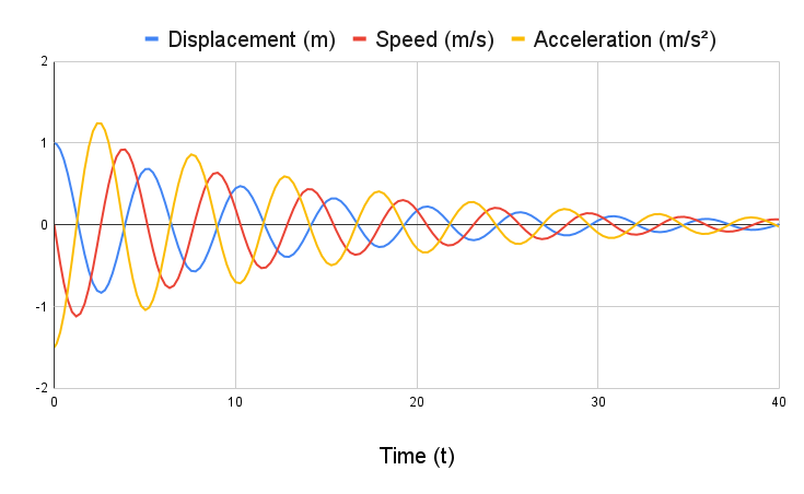
7.8 Genetic Algorithm Software
7.8.1 Implementation
Evolution (/software/evolution.h) is a template class that encapsulates the logic related to GA. Note that this template must be of a class that is a child of the Creature (/software/creature.h) abstract class (interface).
7.8.2 Usage
Arbitrary problem
To perform an optimization using GA, the first step is to define a
child class of Creature
(/software/creature.h). The only definitions required are the
dna attribute and the GetCost function. C
(/software/creature_test.h) class is an example. The creature class,
in this example, represents a candidate \(\{x,y\}\) pair that minimizes \(f(x,y) = x^2 + y^2 + 2x + y\).
Once the child creature class is defined, an
Evolution object can be instantiated and used to search for
optimal solutions. EvolveTest
(/software/evolution_test.cc) contains an example of how that’s
done.
COP
E-GA
The child class for CMs is already defined at ProblemCreature (/software/problem_creature.h). Its constructor uses an auxiliary class ProblemDescription (/software/problem_description.h), which allows us to easily describe a COP as described in sec. 3.2. The extra two parameters from its constructor specify the mass whose maximum acceleration we want to minimize and the length of the simulation we’ll perform. The creature’s loss function is the maximum absolute acceleration that mass will suffer during the dynamic simulation.
P-GA
This
alternative constructor receives Pimodels as dependencies.
If this constructor is used, the Pimodels are used to calculate the
maximum acceleration that the target mass will suffer.
E-GA Example
EvolutionUntilConvergenceTest
(/software/problem_creature_test.cc) contains an example in which we
find values for the springs and dampers of system at fig. 1 that minimize the maximum acceleration
that \(m_5\) would suffer if the system
was moving with a constant speed from right to left and hit an immovable
wall on the left. A simplified version of the code is listed below. Note
that the parameters we pass to the Evolve method determine
our stop condition and if the results should be printed to
stdout. Some values of the best solution found are listed
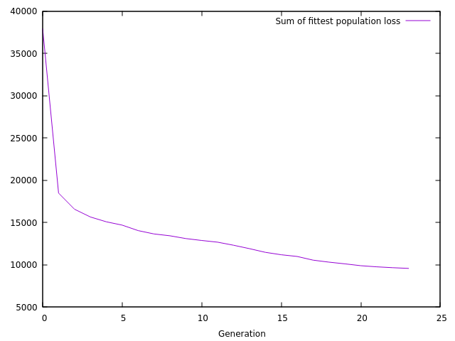
after it, and fig. 9 shows how the sum of the
loss of the fittest population progresses with the generations.
ProblemDescription pd = ProblemDescription();
pd.AddMass(1.0, 0.0, 0.0);  // m0
pd.AddMass(300, 1.0, 1.0);  // m1
pd.AddMass(120, 1.0, 0.0);  // m2
pd.AddMass(150, 1.0, 3.0);  // m3
pd.AddMass(700, 2.0, 0.0);  // m4
pd.AddMass(80, 3.0, 0.0);   // m5

double min = 100.0;
double max = 100000;
pd.AddSpring(0, 1, min, max);
pd.AddSpring(1, 2, min, max);
pd.AddSpring(1, 3, min, max);
pd.AddSpring(1, 4, min, max);
pd.AddDamper(1, 4, min, max);
pd.AddSpring(0, 2, min, max);
pd.AddDamper(0, 2, min, max);
pd.AddSpring(2, 4, min, max);
pd.AddDamper(2, 4, min, max);
pd.AddSpring(0, 3, min, max);
pd.AddDamper(0, 3, min, max);
pd.AddSpring(3, 4, min, max);
pd.AddDamper(3, 4, min, max);
pd.AddSpring(4, 5, min, max);
pd.AddDamper(4, 5, min, max);

pd.SetFixedMass(0);
pd.AddInitialVel(200.0);

// Create population of 20 creatures
std::vector<ProblemCreature> pop = std::vector<ProblemCreature>();
for (int i = 0; i < 20; i++) {
    pop.push_back(ProblemCreature(&pd, 5, 0.15));
}

// Find optimal solutions
Evolution<ProblemCreature> evolution = Evolution<ProblemCreature>(&pop);
double cost0 = evolution.FittestCost();
auto p = evolution.Evolve(0.01, true);

// Check values of best solution
Problem best = pd.BuildFromDNA(evolution.GetCreature(0)->dna).val;
print("k1: ", best.springs[0].Get_k());
print("k2: ", best.springs[1].Get_k());
print("k3: ", best.springs[2].Get_k());
print("k4: ", best.springs[3].Get_k());
print("c4: ", best.dampers[0].Get_c());
print("k5: ", best.springs[4].Get_k());
print("c5: ", best.dampers[1].Get_c());
Some of the values of springs and dampers of the optimal solution we found are:
| Component | Value |
|---|---|
| k1 | 28870.3 |
| k2 | 73618 |
| k3 | 43417.4 |
| k4 | 70919.7 |
| c4 | 4957.4 |
| k5 | 21287.2 |
| c5 | 4957.4 |
7.9 Experiments
Problems
To compare the E-GA and the P-GA approaches, we solved some COPs of different complexities using each method, and then compared the results and the performance of each. The COPs that were solved were all of fully connected systems, i.e. made up of set of masses that are all connected to each other with a spring and a damper. The following code shows how these problems were constructed:
ProblemDescription pd = ProblemDescription();
pd.AddMass(1.0, 0.0, 0.0);  // m0 is fixed
pd.SetFixedMass(0);

for (int i = 1; i <= nMasses; i++) {
    pd.AddMass(Random(100, 300), i, 0);
}
double min = 100000.0;
double max = 300000.0;
for (int i = 0; i < nMasses; i++) {
    for (int j = i + 1; j <= nMasses; j++) {
        pd.AddSpring(i, j, min, max);
        pd.AddDamper(i, j, min, max);
    }
}
for (int i = 1; i <= nMasses; i++) {
    pd.AddInitialVel(i, Random(0.0, 200.0));
    pd.AddInitialDisp(i, Random(0.0, 200.0));
}
Note that the characteristics of the problems (the masses, the
initial conditions and the max/min values of the springs and dampers)
are randomly created, so for each value of nMasses from
1 to 5, 3 random problems were
solved with each approach (E-GA and P-GA), as shown in the pseudo-code
snippet bellow:
for (int problemId = 0; problemId < 3; problemId++) {
    for (int nMasses = 1; nMasses <= 5; nMasses++) {
        optimizeRandomProblemWithEgaAndPga(nMasses);
    }
}
See the full code and the values of all the hyperparameters at /software/experiment_1.cc
7.9.2 Metrics
Both approaches (E-GA and P-GA) start with an initial pool of random guesses. Besides both approaches, we also analyzed the results of the best of those initial random guesses. The best random guess was determined by simply evaluating all the initial guesses with Explicit Time Integration, since that provides the most accurate result. To ensure a fair comparison between the approaches, we ensured that E-GA and P-GA start with the same initial random guesses.
To be able to compare both performance and quality of each approach, for each problem solved a score from 0 to 100 was given to the efficiency and quality of E-GA, P-GA and of the Best Initial Random Guess. The efficiency was simply measured by the time the algorithm took to run. The quality was measured by how small the maximum acceleration of the target mass was during the impact for each solution. The acceleration was determined once again with the Explicit Time Integration for a fair comparison between E-GA and P-GA.
An efficiency score of 100 means that that particular approach was the fastest among the three. A score of 0 means that approach was the slowest. A value in between is the result of an interpolation between the maximum and minimum execution time. The quality score is analogous. The results are shown in sec. 5.2.
7.9.3 Hyperparameters
A very important note is that the hyperparameters have been carefully chosen, through experimentation an trial and error, so that the P-GA would reach good results with a execution time comparable to the E-GA. See sec. 6 for more details.
8 Results
8.1 PIM
8.1.1 Simple harmonic oscillator
fig. 10 shows the result of TrainTest
/software/pimodel_test.cc, which tests how well PIMs can approximate a solution obtained
with Explicit Time Integration. The COP for which the PIMs were trained consists on a system of
two masses attached by a spring and a damper. One of the masses is fixed
and the other has an initial displacement. The models used have
order=3, and a TimeDiscretization=8 was
used.
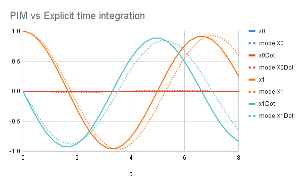
The results show that the PIMs very closely approximate the solution obtained by the ETI method.
8.1.2 Larger system
fig. 11 shows the result of /software/pimodel_binary_test.cc.
This tests is very similar to sec. 5.1.1, but the COP
at hand is much larger. It’s a system of 5 masses, 9 springs and 6
dampers. One of the masses is fixed, and all the other ones start with
an initial velocity. The models used have order=3, and a
TimeDiscretization=20 was used.
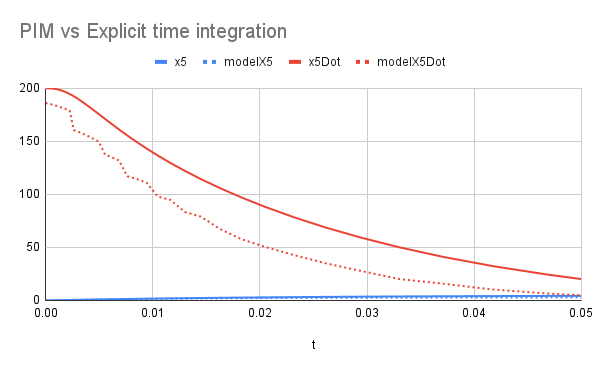
These results show once again that the PIMs very closely approximate the solution obtained by the ETI method.
8.2 E-GA vs P-GA vs Random
The following table shows the Efficiency and Quality scores of the tests performed. The first column indicates the number of non-fixed masses of the system, and the second indicates the “id” of the experiment (3 random COPs were solved for each number of non-fixed masses). See sec. 4.9 for context.
| Masses | Test | Method | Efficiency score | Quality score | Mean score |
|---|---|---|---|---|---|
| 1 | 0 | P-GA | 34.3654 | 71.0724 | 52.7189 |
| 1 | 0 | E-GA | 0 | 100 | 50 |
| 1 | 0 | Random Guess | 100 | 0 | 50 |
| 1 | 1 | P-GA | 75.6739 | 0 | 37.837 |
| 1 | 1 | E-GA | 0 | 100 | 50 |
| 1 | 1 | Random Guess | 100 | 0 | 50 |
| 1 | 2 | P-GA | 28.472 | 90.0197 | 59.2458 |
| 1 | 2 | E-GA | 0 | 100 | 50 |
| 1 | 2 | Random Guess | 100 | 0 | 50 |
| 2 | 0 | P-GA | 72.3782 | 67.4949 | 69.9366 |
| 2 | 0 | E-GA | 0 | 100 | 50 |
| 2 | 0 | Random Guess | 100 | 0 | 50 |
| 2 | 1 | P-GA | 47.5716 | 99.0683 | 73.3199 |
| 2 | 1 | E-GA | 0 | 100 | 50 |
| 2 | 1 | Random Guess | 100 | 0 | 50 |
| 2 | 2 | P-GA | 62.6595 | 100 | 81.3298 |
| 2 | 2 | E-GA | 0 | 98.1363 | 49.0681 |
| 2 | 2 | Random Guess | 100 | 0 | 50 |
| 3 | 0 | P-GA | 78.3921 | 60.019 | 69.2055 |
| 3 | 0 | E-GA | 0 | 100 | 50 |
| 3 | 0 | Random Guess | 100 | 0 | 50 |
| 3 | 1 | P-GA | 67.7193 | 42.6812 | 55.2003 |
| 3 | 1 | E-GA | 0 | 100 | 50 |
| 3 | 1 | Random Guess | 100 | 0 | 50 |
| 3 | 2 | P-GA | 79.8498 | 16.795 | 48.3224 |
| 3 | 2 | E-GA | 0 | 100 | 50 |
| 3 | 2 | Random Guess | 100 | 0 | 50 |
| 4 | 0 | P-GA | 82.5093 | 0 | 41.2546 |
| 4 | 0 | E-GA | 0 | 100 | 50 |
| 4 | 0 | Random Guess | 100 | 35.6312 | 67.8156 |
| 4 | 1 | P-GA | 64.3856 | 80.9193 | 72.6525 |
| 4 | 1 | E-GA | 0 | 100 | 50 |
| 4 | 1 | Random Guess | 100 | 0 | 50 |
| 4 | 2 | P-GA | 65.827 | 70.105 | 67.966 |
| 4 | 2 | E-GA | 0 | 100 | 50 |
| 4 | 2 | Random Guess | 100 | 0 | 50 |
| 5 | 0 | P-GA | 85.4621 | 27.0249 | 56.2435 |
| 5 | 0 | E-GA | 0 | 100 | 50 |
| 5 | 0 | Random Guess | 100 | 0 | 50 |
| 5 | 1 | P-GA | 84.2239 | 23.8868 | 54.0554 |
| 5 | 1 | E-GA | 0 | 100 | 50 |
| 5 | 1 | Random Guess | 100 | 0 | 50 |
| 5 | 2 | P-GA | 44.2273 | 15.1486 | 29.6879 |
| 5 | 2 | E-GA | 0 | 100 | 50 |
| 5 | 2 | Random Guess | 100 | 0 | 50 |
The results show that in many cases the P-GA can obtain
solutions which are very close or even better than the ones obtained by
the E-GA; but that’s not always the case. In some cases,
P-GA can even lead to results which are significantly worse
than the E-GA ones and possibly even worse than random
guesses (see {Masses=4,Test=0}).
8.3 Conclusions
Especially given that the hyperparameters have been carefully chosen
through trial and error (see sec. 4.9.2), we can’t make broad statements
about the efficacy of the using P-GA instead of
E-GA.
Still, the results do show some very promising results because we see many cases in which the usage of Physics Informed Machine Learning Models in the Genetic Algorithm brought results as good as the Genetic Algorithm that performs numerical integration to evaluate the fitness of solutions; but in in a much smaller execution time.
The results are not at all generalizable, but they definitely show a great potential in using Physics Informed Machine Learning Models as solution-fitness estimators for performance gains.
9 Discussion
In this work, we explored the potential of Physics-Informed Machine Learning Models (PIMs) to increase the efficiency of Genetic Algorithms (GAs) for the optimization of mechanical systems. Traditionally, these GAs use numerical simulations (such as Explicit Time Integration or the Finite Element Method) to measure the fitness of each candidate solution. These numerical simulations can be quite expensive and become computational bottlenecks, but - once trained - PIMs can rapidly estimate the fitness of candidates. The training of these models is, however, not free; so at first glance it’s not easy to say if using them is indeed efficient or not.
Our investigations revealed many cases in which PIM-enhanced GA yielded substantial time savings when compared to the Numerical GA (which uses Explicit Time Integration to evaluate each candidate solution). Moreover, we saw that PIM-enhanced GAs were not only faster but also capable of producing solutions of comparable quality, or even superior quality, to those obtained using the Numerical GA.
In some of the experiments, however, PIM-enhanced GA led to a solution which was worse than a random guess; so it’s not always that this method works. Also, finding the hyperparameters which cause the models to train fast enough while still causing them to be good-enough estimators is tricky and very operator-dependent. Thus, we can’t argue that this is a technique that should always replace Numerical GA.
However, it’s vital to recognize that these findings do not diminish the promise of PIM-enhanced GAs. After all, 11 out of 15 experiments showed not only a much smaller execution time but a larger Mean Score (the mean between the efficiency and the quality score) for the PIM-enhanced GA, and in one case the solution found by the PIM-enhanced GA was even better than the one found by the Numerical GA. Some clear follow-up questions worthy of investigation are:
How does the performance of the technique changes with more refined models? We only used simple linear models, so it stands to question if more refined models can be trained faster but reach the same inference quality.
How does it perform in other mechanical problems? We only analyzed systems made up of masses springs and dampers, but the technique can easily be applied to other problems as well.
What are the optimal hyperparameters for the training? How do we find them for each specific problem?
In conclusion, our work establishes a compelling case for further research about the incorporation of Physics-Informed Machine Learning Models into GAs to dramatically enhance optimization performance. This approach not only holds the potential to significantly accelerate solution searches but also to maintain or even improve solution quality, which can unlock possibilities for tackling previously intractable problems across a multitude of disciplines.